Python Geospatial Libraries

Interactive Jupyter Notebook

This notebook provides an introduction to Python Geospatial Libraries, mainly GeoPandas (including aspects of Pandas), and Shapely. This notebook was created by Becky Vandewalle based off of prior work by Dandong Yin.

Introduction

Pandas is a Python library for data analysis, featuring easy IO, powerful indexing, database operations, and categorical data support. Two primary data structures in Pandas are `Series` and `DataFrame`.

GeoPandas extends Pandas by adding core geographical functionality. You can do spatial database-like operations with this library.

Shapely is useful for working with vector data using set-like operators.

Setup

Run this cell for the rest of the notebook to work!

In [8]:
# import required libraries

%matplotlib inline
import os
import geopandas as gpd
import pandas as pd
import numpy as np
import shapely

Import Data

The main dataset used in this notebook is stored as a dBase database file (.dbf). Pandas can not import a dBase file directly, so Geopandas is used to convert it to a format Pandas can read.

In [9]:
# import towns database

towns_temp_gpd = gpd.read_file(os.path.join('./pyintro_resources/data','towns.dbf'))
towns_table = pd.DataFrame(towns_temp_gpd)[:10]


countries = gpd.read_file(os.path.join(r'zip://pyintro_resources/data/ne_10m_admin_0_countries.zip'))
cities = gpd.read_file(os.path.join(r'zip://pyintro_resources/data/ne_10m_populated_places.zip'))
rivers = gpd.read_file(os.path.join(r'zip://pyintro_resources/data/ne_10m_rivers_lake_centerlines.zip'))

# check type

type(towns_table)
Out[9]:
pandas.core.frame.DataFrame

Lets check to make sure the data were properly loaded by looking at the first few rows containing town information (more on the head and tail functions later).

In [10]:
# show initial values of data frame

towns_table.head()
Out[10]:
TOWN_ID TOWN FIPS_STCO CCD_MCD FIPS_PLACE POP1980 POP1990 POP2000 POPCH80_90 POPCH90_00 FOURCOLOR TYPE POP2010 POPCH00_10 SHAPE_AREA SHAPE_LEN geometry
0 195 MOUNT WASHINGTON 25003 080 43300 100 135 130 35 -5 1 T 167 37 5.797118e+07 31638.316048 POLYGON ((36115.894 880179.251, 36980.214 8796...
1 325 WEST SPRINGFIELD 25013 110 76030 26965 27537 27899 572 362 2 TC 28391 492 4.531454e+07 34458.401293 POLYGON ((106810.684 879681.441, 106814.824 87...
2 122 HANOVER 25023 040 28285 11403 11912 13164 509 1252 1 T 13879 715 4.059553e+07 29602.365447 POLYGON ((250886.704 878325.941, 251695.934 87...
3 18 AVON 25021 005 02935 4843 4558 4443 -285 -115 4 T 4356 -87 1.174804e+07 14941.830951 POLYGON ((238434.144 876232.691, 239075.264 87...
4 112 GRANVILLE 25013 035 26675 1298 1403 1521 105 118 4 T 1566 45 1.115403e+08 43612.600436 POLYGON ((77501.874 877293.751, 83945.044 8759...

We will return to the towns database later. For now, lets start by exploring a Series.

Introducing the Series

A Series in Pandas is a one-dimensional labeled array capable of holding a wide variety of data. This array also has an index, which is like a label for each of the values in the array. The basic method to create a Series is to call:

pd.Series(data, index=index)

Here, data can be many different things, such as:

  • a Python dictionary
  • a numpy array
  • a scalar value (like 5)

Anything like an array, iterable, a dictionary, or a scalar value, will work for data contents!

Basically, a Series is a list with an index!

Here are some examples of constructing a `Series`:

In [11]:
# create a basic series

pd.Series([0,1,2], index=['a', 'b', 'c'])
Out[11]:
a    0
b    1
c    2
dtype: int64

Note that index values are on the left.

In [12]:
# create a series using a dictionary of values and index values

pd.Series({'a' : 0, 'b' : 1, 'c' : 2})
Out[12]:
a    0
b    1
c    2
dtype: int64
In [13]:
# scalar values will be repeated to be the length of the index

pd.Series(5, index=['a', 'b', 'c'])
Out[13]:
a    5
b    5
c    5
dtype: int64
In [14]:
# but the opposite does not work
# this cell will fail to run!

pd.Series([5, 5, 5], index=['a'])
---------------------------------------------------------------------------
ValueError                                Traceback (most recent call last)
<ipython-input-14-de84def1995a> in <module>
      2 # this cell will fail to run!
      3 
----> 4 pd.Series([5, 5, 5], index=['a'])

/opt/conda/lib/python3.7/site-packages/pandas/core/series.py in __init__(self, data, index, dtype, name, copy, fastpath)
    300                         raise ValueError(
    301                             "Length of passed values is {val}, "
--> 302                             "index implies {ind}".format(val=len(data), ind=len(index))
    303                         )
    304                 except TypeError:

ValueError: Length of passed values is 3, index implies 1
In [15]:
# if no index is provided, data values will be used as an index

pd.Series([0,1,2])
Out[15]:
0    0
1    1
2    2
dtype: int64

Once you have a series object you can access the data and index values directly:

In [16]:
# see type of series

myseries = pd.Series({'a' : 0, 'b' : 1, 'c' : 2})
type(myseries)
Out[16]:
pandas.core.series.Series
In [17]:
# list series values

list(myseries.values)
Out[17]:
[0, 1, 2]
In [18]:
# list series index values

list(myseries.index)
Out[18]:
['a', 'b', 'c']

Array-like Behavior

You can access elements of a `Series` using the index operator, just like for regular lists and tuples in Python. Remember that Python indices start with 0.

Here are a few examples:

In [19]:
# return the first element

myseries[0]
Out[19]:
0
In [20]:
# select everything up until element index 2 (the third element)

myseries[:2]
Out[20]:
a    0
b    1
dtype: int64
In [21]:
# find the median value

myseries.median()
Out[21]:
1.0

Operations can be performed element-wise for the series.

In [22]:
# see which elements are greater than the medium

myseries > myseries.median()
Out[22]:
a    False
b    False
c     True
dtype: bool

Use any or all to check if a comparison is true for the series as a whole.

In [23]:
# are any elements greater than the medium value?

any(myseries > myseries.median())
Out[23]:
True
In [24]:
# are all elements greater than the medium value?

all(myseries > myseries.median())
Out[24]:
False

You can also select values using a logical index series.

In [25]:
# select by greater than median

myseries[myseries > myseries.median()]
Out[25]:
c    2
dtype: int64
In [26]:
myseries
Out[26]:
a    0
b    1
c    2
dtype: int64

You can also pass a list of indices to select series elements out of order.

In [27]:
# select by list of indices

myseries[[2, 1, 1]]
Out[27]:
c    2
b    1
b    1
dtype: int64

Other operations are performed element-wise too. For example:

In [28]:
# add series values to self

myseries + myseries
Out[28]:
a    0
b    2
c    4
dtype: int64
In [29]:
# raise to the 3rd power

myseries ** 3
Out[29]:
a    0
b    1
c    8
dtype: int64

Dictionary-like Behavior

Since a `Series` has an index, you can also work with a Series as if it were a Python dictionary:

In [30]:
# find value with index 'a'

myseries['a']
Out[30]:
0
In [31]:
# set value of 'd'

myseries['d'] = 5
myseries
Out[31]:
a    0
b    1
c    2
d    5
dtype: int64
In [32]:
# see if index value in series

'f' in myseries
Out[32]:
False
In [33]:
# see if index value in series

'c' in myseries
Out[33]:
True

'Naming' a series

A Series has an optional `name` parameter:

In [34]:
# see current name (not assigned)

print (myseries.name)
None

If you name a Series, the name will show up in the information at the bottom:

In [35]:
# set name

myseries.rename('stock_price')
Out[35]:
a    0
b    1
c    2
d    5
Name: stock_price, dtype: int64

Introducing the DataFrame

What happens when a Series gains a dimension? It becomes a `DataFrame`!

We can use the towns database we imported at the beginning of this Notebook to see how to check out a DataFrame. The head function is useful to see the first few rows of a DataFrame.

In [36]:
# see start of DataFrame

towns_table.head()
Out[36]:
TOWN_ID TOWN FIPS_STCO CCD_MCD FIPS_PLACE POP1980 POP1990 POP2000 POPCH80_90 POPCH90_00 FOURCOLOR TYPE POP2010 POPCH00_10 SHAPE_AREA SHAPE_LEN geometry
0 195 MOUNT WASHINGTON 25003 080 43300 100 135 130 35 -5 1 T 167 37 5.797118e+07 31638.316048 POLYGON ((36115.894 880179.251, 36980.214 8796...
1 325 WEST SPRINGFIELD 25013 110 76030 26965 27537 27899 572 362 2 TC 28391 492 4.531454e+07 34458.401293 POLYGON ((106810.684 879681.441, 106814.824 87...
2 122 HANOVER 25023 040 28285 11403 11912 13164 509 1252 1 T 13879 715 4.059553e+07 29602.365447 POLYGON ((250886.704 878325.941, 251695.934 87...
3 18 AVON 25021 005 02935 4843 4558 4443 -285 -115 4 T 4356 -87 1.174804e+07 14941.830951 POLYGON ((238434.144 876232.691, 239075.264 87...
4 112 GRANVILLE 25013 035 26675 1298 1403 1521 105 118 4 T 1566 45 1.115403e+08 43612.600436 POLYGON ((77501.874 877293.751, 83945.044 8759...

Similarly, the tail function can be used to check the end:

In [37]:
# see end of DataFrame

towns_table.tail()
Out[37]:
TOWN_ID TOWN FIPS_STCO CCD_MCD FIPS_PLACE POP1980 POP1990 POP2000 POPCH80_90 POPCH90_00 FOURCOLOR TYPE POP2010 POPCH00_10 SHAPE_AREA SHAPE_LEN geometry
5 231 PEMBROKE 25023 095 52630 13882 14544 16927 662 2383 4 T 17837 910 6.100425e+07 42214.822703 POLYGON ((259776.144 874290.371, 259957.504 87...
6 304 UXBRIDGE 25027 260 71620 8621 10415 11156 1794 741 2 T 13457 2301 7.766001e+07 39595.624547 POLYGON ((192331.674 873780.751, 192392.504 86...
7 5 AGAWAM 25013 005 00800 26754 27323 28144 569 821 4 TC 28438 294 6.319876e+07 38160.729223 POLYGON ((109952.354 871999.621, 110162.394 87...
8 120 HAMPDEN 25013 040 28075 4665 4709 5171 44 462 4 T 5139 -32 5.099855e+07 29454.532879 POLYGON ((127256.784 872905.191, 127635.434 86...
9 88 EASTON 25005 030 20100 17719 19807 22299 2088 2492 4 T 23112 813 7.571470e+07 36051.552667 POLYGON ((234696.174 871764.311, 235620.094 86...

Like a Series, a DataFrame has an index. This one is a numeric range.

In [38]:
# see index

towns_table.index
Out[38]:
RangeIndex(start=0, stop=10, step=1)

You can also list the DataFrame column names:

In [39]:
# see column names

towns_table.columns
Out[39]:
Index(['TOWN_ID', 'TOWN', 'FIPS_STCO', 'CCD_MCD', 'FIPS_PLACE', 'POP1980',
       'POP1990', 'POP2000', 'POPCH80_90', 'POPCH90_00', 'FOURCOLOR', 'TYPE',
       'POP2010', 'POPCH00_10', 'SHAPE_AREA', 'SHAPE_LEN', 'geometry'],
      dtype='object')

And it is often useful to dig into its values:

In [40]:
# see values

towns_table.values
Out[40]:
array([[195, 'MOUNT WASHINGTON', 25003, '080', '43300', 100, 135, 130,
        35, -5, 1, 'T', 167, 37, 57971179.2348, 31638.3160483,
        <shapely.geometry.polygon.Polygon object at 0x7f0aaeab8f28>],
       [325, 'WEST SPRINGFIELD', 25013, '110', '76030', 26965, 27537,
        27899, 572, 362, 2, 'TC', 28391, 492, 45314535.7868,
        34458.4012926,
        <shapely.geometry.polygon.Polygon object at 0x7f0aaeb2b438>],
       [122, 'HANOVER', 25023, '040', '28285', 11403, 11912, 13164, 509,
        1252, 1, 'T', 13879, 715, 40595530.4619, 29602.3654467,
        <shapely.geometry.polygon.Polygon object at 0x7f0ae8444400>],
       [18, 'AVON', 25021, '005', '02935', 4843, 4558, 4443, -285, -115,
        4, 'T', 4356, -87, 11748038.1104, 14941.8309508,
        <shapely.geometry.polygon.Polygon object at 0x7f0aaea8c898>],
       [112, 'GRANVILLE', 25013, '035', '26675', 1298, 1403, 1521, 105,
        118, 4, 'T', 1566, 45, 111540272.728, 43612.6004363,
        <shapely.geometry.polygon.Polygon object at 0x7f0aaea82048>],
       [231, 'PEMBROKE', 25023, '095', '52630', 13882, 14544, 16927, 662,
        2383, 4, 'T', 17837, 910, 61004248.7947, 42214.8227033,
        <shapely.geometry.polygon.Polygon object at 0x7f0aaea82b00>],
       [304, 'UXBRIDGE', 25027, '260', '71620', 8621, 10415, 11156, 1794,
        741, 2, 'T', 13457, 2301, 77660011.8388, 39595.6245467,
        <shapely.geometry.polygon.Polygon object at 0x7f0aaeb153c8>],
       [5, 'AGAWAM', 25013, '005', '00800', 26754, 27323, 28144, 569,
        821, 4, 'TC', 28438, 294, 63198758.6208, 38160.7292232,
        <shapely.geometry.polygon.Polygon object at 0x7f0aaeb15cf8>],
       [120, 'HAMPDEN', 25013, '040', '28075', 4665, 4709, 5171, 44, 462,
        4, 'T', 5139, -32, 50998545.098, 29454.532879,
        <shapely.geometry.polygon.Polygon object at 0x7f0aaeb15860>],
       [88, 'EASTON', 25005, '030', '20100', 17719, 19807, 22299, 2088,
        2492, 4, 'T', 23112, 813, 75714695.8844, 36051.5526666,
        <shapely.geometry.polygon.Polygon object at 0x7f0aaea892b0>]],
      dtype=object)

It can be useful to double check the size of the values array. We know from the index that there are 351 rows, and now we can see there are 17 columns (by a few different methods).

In [41]:
# see the size of the values array

towns_table.values.shape
Out[41]:
(10, 17)
In [42]:
# count columns

print (len(towns_table.values[0]))
print (len(towns_table.columns))
17
17

Using index selection we can see all values in one row.

In [43]:
# see one row

towns_table.values[5]
Out[43]:
array([231, 'PEMBROKE', 25023, '095', '52630', 13882, 14544, 16927, 662,
       2383, 4, 'T', 17837, 910, 61004248.7947, 42214.8227033,
       <shapely.geometry.polygon.Polygon object at 0x7f0aaea82b00>],
      dtype=object)

We can use the double index method to find a value within a particular and row and column:

In [44]:
# find specific value

towns_table.values[5][5]
Out[44]:
13882

Sometimes it is useful to know summary information about a DataFrame. The describe makes this clear:

In [45]:
# summarize DataFrame

towns_table.describe()
Out[45]:
TOWN_ID FIPS_STCO POP1980 POP1990 POP2000 POPCH80_90 POPCH90_00 FOURCOLOR POP2010 POPCH00_10 SHAPE_AREA SHAPE_LEN
count 10.000000 10.000000 10.000000 10.000000 10.000000 10.000000 10.000000 10.000000 10.000000 10.000000 1.000000e+01 10.000000
mean 152.000000 25015.400000 11625.000000 12234.300000 13085.400000 609.300000 851.100000 3.000000 13634.200000 548.800000 5.957458e+07 33973.077619
std 109.700603 7.933053 9714.914673 10039.928984 10480.075267 768.070895 931.386595 1.333333 10696.622175 716.749422 2.631064e+07 8311.382105
min 5.000000 25003.000000 100.000000 135.000000 130.000000 -285.000000 -115.000000 1.000000 167.000000 -87.000000 1.174804e+07 14941.830951
25% 94.000000 25013.000000 4709.500000 4595.750000 4625.000000 59.250000 179.000000 2.000000 4551.750000 39.000000 4.673554e+07 30111.353097
50% 121.000000 25013.000000 10012.000000 11163.500000 12160.000000 539.000000 601.500000 4.000000 13668.000000 393.000000 5.948771e+07 35254.976980
75% 222.000000 25022.500000 16759.750000 18491.250000 20956.000000 639.500000 1144.250000 4.000000 21793.250000 788.500000 7.258571e+07 39236.900716
max 325.000000 25027.000000 26965.000000 27537.000000 28144.000000 2088.000000 2492.000000 4.000000 28438.000000 2301.000000 1.115403e+08 43612.600436

Transposing a DataFrame can also come in handy:

In [46]:
# transpose DataFrame

towns_table.T
Out[46]:
0 1 2 3 4 5 6 7 8 9
TOWN_ID 195 325 122 18 112 231 304 5 120 88
TOWN MOUNT WASHINGTON WEST SPRINGFIELD HANOVER AVON GRANVILLE PEMBROKE UXBRIDGE AGAWAM HAMPDEN EASTON
FIPS_STCO 25003 25013 25023 25021 25013 25023 25027 25013 25013 25005
CCD_MCD 080 110 040 005 035 095 260 005 040 030
FIPS_PLACE 43300 76030 28285 02935 26675 52630 71620 00800 28075 20100
POP1980 100 26965 11403 4843 1298 13882 8621 26754 4665 17719
POP1990 135 27537 11912 4558 1403 14544 10415 27323 4709 19807
POP2000 130 27899 13164 4443 1521 16927 11156 28144 5171 22299
POPCH80_90 35 572 509 -285 105 662 1794 569 44 2088
POPCH90_00 -5 362 1252 -115 118 2383 741 821 462 2492
FOURCOLOR 1 2 1 4 4 4 2 4 4 4
TYPE T TC T T T T T TC T T
POP2010 167 28391 13879 4356 1566 17837 13457 28438 5139 23112
POPCH00_10 37 492 715 -87 45 910 2301 294 -32 813
SHAPE_AREA 5.79712e+07 4.53145e+07 4.05955e+07 1.1748e+07 1.1154e+08 6.10042e+07 7.766e+07 6.31988e+07 5.09985e+07 7.57147e+07
SHAPE_LEN 31638.3 34458.4 29602.4 14941.8 43612.6 42214.8 39595.6 38160.7 29454.5 36051.6
geometry POLYGON ((36115.89421539754 880179.2508560009,... POLYGON ((106810.6842153966 879681.4408560023,... POLYGON ((250886.7042153999 878325.9408560023,... POLYGON ((238434.1442153975 876232.6908560023,... POLYGON ((77501.87421539426 877293.7508560009,... POLYGON ((259776.1442153975 874290.370856002, ... POLYGON ((192331.6742153987 873780.7508560009,... POLYGON ((109952.3542153984 871999.620856002, ... POLYGON ((127256.7842153981 872905.1908560023,... POLYGON ((234696.1742153987 871764.3108559996,...

It is also possible to sort a DataFrame by values in a particular column:

In [47]:
# sort DataFrame by column

towns_table.sort_values(by='POP2010')
Out[47]:
TOWN_ID TOWN FIPS_STCO CCD_MCD FIPS_PLACE POP1980 POP1990 POP2000 POPCH80_90 POPCH90_00 FOURCOLOR TYPE POP2010 POPCH00_10 SHAPE_AREA SHAPE_LEN geometry
0 195 MOUNT WASHINGTON 25003 080 43300 100 135 130 35 -5 1 T 167 37 5.797118e+07 31638.316048 POLYGON ((36115.894 880179.251, 36980.214 8796...
4 112 GRANVILLE 25013 035 26675 1298 1403 1521 105 118 4 T 1566 45 1.115403e+08 43612.600436 POLYGON ((77501.874 877293.751, 83945.044 8759...
3 18 AVON 25021 005 02935 4843 4558 4443 -285 -115 4 T 4356 -87 1.174804e+07 14941.830951 POLYGON ((238434.144 876232.691, 239075.264 87...
8 120 HAMPDEN 25013 040 28075 4665 4709 5171 44 462 4 T 5139 -32 5.099855e+07 29454.532879 POLYGON ((127256.784 872905.191, 127635.434 86...
6 304 UXBRIDGE 25027 260 71620 8621 10415 11156 1794 741 2 T 13457 2301 7.766001e+07 39595.624547 POLYGON ((192331.674 873780.751, 192392.504 86...
2 122 HANOVER 25023 040 28285 11403 11912 13164 509 1252 1 T 13879 715 4.059553e+07 29602.365447 POLYGON ((250886.704 878325.941, 251695.934 87...
5 231 PEMBROKE 25023 095 52630 13882 14544 16927 662 2383 4 T 17837 910 6.100425e+07 42214.822703 POLYGON ((259776.144 874290.371, 259957.504 87...
9 88 EASTON 25005 030 20100 17719 19807 22299 2088 2492 4 T 23112 813 7.571470e+07 36051.552667 POLYGON ((234696.174 871764.311, 235620.094 86...
1 325 WEST SPRINGFIELD 25013 110 76030 26965 27537 27899 572 362 2 TC 28391 492 4.531454e+07 34458.401293 POLYGON ((106810.684 879681.441, 106814.824 87...
7 5 AGAWAM 25013 005 00800 26754 27323 28144 569 821 4 TC 28438 294 6.319876e+07 38160.729223 POLYGON ((109952.354 871999.621, 110162.394 87...

From Series to DataFrame

Now that we are slightly more familiar with the DataFrame, we can go into more detail. Technically, a DataFrame is implemented as a list of named Series all with the same index values.

In [48]:
# construct a DataFrame

myDataFrame = pd.DataFrame(
    {'one' : pd.Series([1., 2., 3.], index=['a', 'b', 'c']),
     'two' : pd.Series([1., 2., 3., 4.], index=['a', 'b', 'c', 'd'])})

myDataFrame
Out[48]:
one two
a 1.0 1.0
b 2.0 2.0
c 3.0 3.0
d NaN 4.0

Remember the name attribute for a Series? Since each column in a DataFrame is a Series, each column name is equivalent to the name of the Series for that column.

In [49]:
# show DataFrame column names

myDataFrame.columns
Out[49]:
Index(['one', 'two'], dtype='object')

Manipulating a DataFrame

Columns in a DataFrame can be freely selected, added, deleted (as with the "dictionary" aspect of Series):

In [50]:
# create new column from existing columns

myDataFrame['three'] = myDataFrame['one'] + myDataFrame['two']
myDataFrame
Out[50]:
one two three
a 1.0 1.0 2.0
b 2.0 2.0 4.0
c 3.0 3.0 6.0
d NaN 4.0 NaN

Columns in a DataFrame do not have to all be the same data type (as we saw with the towns database):

In [51]:
# create new column from comparison

myDataFrame['flag'] = myDataFrame['one'] > 2
myDataFrame
Out[51]:
one two three flag
a 1.0 1.0 2.0 False
b 2.0 2.0 4.0 False
c 3.0 3.0 6.0 True
d NaN 4.0 NaN False

It is simple to delete a column:

In [52]:
# delete column

del myDataFrame['two']
myDataFrame
Out[52]:
one three flag
a 1.0 2.0 False
b 2.0 4.0 False
c 3.0 6.0 True
d NaN NaN False

Scalar values assigned to a column repeat to fit the length of the DataFrame.

In [53]:
# add column

myDataFrame['four'] = 4
myDataFrame
Out[53]:
one three flag four
a 1.0 2.0 False 4
b 2.0 4.0 False 4
c 3.0 6.0 True 4
d NaN NaN False 4

You can also add a new row to the DataFrame using the append function.

In [54]:
# add row to DataFrame

myDataFrame.append({'one':3,'three':2.0,'flag':False},ignore_index=True)
Out[54]:
one three flag four
0 1.0 2.0 False 4.0
1 2.0 4.0 False 4.0
2 3.0 6.0 True 4.0
3 NaN NaN False 4.0
4 3.0 2.0 False NaN

Note that the changes won't affect the original DataFrame unless you re-assign it.

In [55]:
myDataFrame
Out[55]:
one three flag four
a 1.0 2.0 False 4
b 2.0 4.0 False 4
c 3.0 6.0 True 4
d NaN NaN False 4
In [56]:
# add row to DataFrame

myDataFrame2 = myDataFrame.append({'one':3,'three':2.0,'flag':False},ignore_index=True)
In [57]:
myDataFrame2
Out[57]:
one three flag four
0 1.0 2.0 False 4.0
1 2.0 4.0 False 4.0
2 3.0 6.0 True 4.0
3 NaN NaN False 4.0
4 3.0 2.0 False NaN

Don't add rows dynamically too often, as append makes a full copy of the data, so constantly using this function can create a significant performance hit. A better way is to include all rows while creating the DataFrame.

You can also drop rows and columns:

In [58]:
# drop rows

myDataFrame.drop(['a','c'])
Out[58]:
one three flag four
b 2.0 4.0 False 4
d NaN NaN False 4

axis specifies whether you are referring to rows or columns:

In [59]:
# drop columns

myDataFrame.drop(['one','four'], axis=1)
Out[59]:
three flag
a 2.0 False
b 4.0 False
c 6.0 True
d NaN False

Selecting Data in a DataFrame

Selecting data is a common task when dealing with a DataFrames.

Select by Label

As seen before, we can select data using label values.

In [60]:
# select column by index

towns_table['POP2010']
Out[60]:
0      167
1    28391
2    13879
3     4356
4     1566
5    17837
6    13457
7    28438
8     5139
9    23112
Name: POP2010, dtype: int64

We can select just a few rows with index slicing:

In [61]:
# select rows

towns_table[0:3]
Out[61]:
TOWN_ID TOWN FIPS_STCO CCD_MCD FIPS_PLACE POP1980 POP1990 POP2000 POPCH80_90 POPCH90_00 FOURCOLOR TYPE POP2010 POPCH00_10 SHAPE_AREA SHAPE_LEN geometry
0 195 MOUNT WASHINGTON 25003 080 43300 100 135 130 35 -5 1 T 167 37 5.797118e+07 31638.316048 POLYGON ((36115.894 880179.251, 36980.214 8796...
1 325 WEST SPRINGFIELD 25013 110 76030 26965 27537 27899 572 362 2 TC 28391 492 4.531454e+07 34458.401293 POLYGON ((106810.684 879681.441, 106814.824 87...
2 122 HANOVER 25023 040 28285 11403 11912 13164 509 1252 1 T 13879 715 4.059553e+07 29602.365447 POLYGON ((250886.704 878325.941, 251695.934 87...

We can combine row selection using indices and selecting columns using labels using the `loc` function:

In [62]:
# select rows and columns

towns_table.loc[0:2,['POP2010','TOWN']]
Out[62]:
POP2010 TOWN
0 167 MOUNT WASHINGTON
1 28391 WEST SPRINGFIELD
2 13879 HANOVER
In [63]:
# select row and columns

towns_table.loc[3,['POP2010','TOWN','POP1990']] 
Out[63]:
POP2010    4356
TOWN       AVON
POP1990    4558
Name: 3, dtype: object
In [64]:
# select specific value

towns_table.loc[3,'POP2010']
Out[64]:
4356

Select by (only) Position

Column label values are not necessary - you can select values using just indices with the `iloc` function. Here are some examples:

In [65]:
# select row

towns_table.iloc[3]
Out[65]:
TOWN_ID                                                      18
TOWN                                                       AVON
FIPS_STCO                                                 25021
CCD_MCD                                                     005
FIPS_PLACE                                                02935
POP1980                                                    4843
POP1990                                                    4558
POP2000                                                    4443
POPCH80_90                                                 -285
POPCH90_00                                                 -115
FOURCOLOR                                                     4
TYPE                                                          T
POP2010                                                    4356
POPCH00_10                                                  -87
SHAPE_AREA                                           1.1748e+07
SHAPE_LEN                                               14941.8
geometry      POLYGON ((238434.1442153975 876232.6908560023,...
Name: 3, dtype: object
In [66]:
# select some columns from row

towns_table.iloc[3,0:5]
Out[66]:
TOWN_ID          18
TOWN           AVON
FIPS_STCO     25021
CCD_MCD         005
FIPS_PLACE    02935
Name: 3, dtype: object
In [67]:
# select some columns from all rows

towns_table.iloc[:,0:5]
Out[67]:
TOWN_ID TOWN FIPS_STCO CCD_MCD FIPS_PLACE
0 195 MOUNT WASHINGTON 25003 080 43300
1 325 WEST SPRINGFIELD 25013 110 76030
2 122 HANOVER 25023 040 28285
3 18 AVON 25021 005 02935
4 112 GRANVILLE 25013 035 26675
5 231 PEMBROKE 25023 095 52630
6 304 UXBRIDGE 25027 260 71620
7 5 AGAWAM 25013 005 00800
8 120 HAMPDEN 25013 040 28075
9 88 EASTON 25005 030 20100
In [68]:
# select rows and columns

towns_table.iloc[:2,:2]
Out[68]:
TOWN_ID TOWN
0 195 MOUNT WASHINGTON
1 325 WEST SPRINGFIELD

Select by Condition

We can use conditional operators to select DataFrame slices that meet specific conditions. Here are examples:

In [69]:
# select by condition

towns_table['POP2010']>16000
Out[69]:
0    False
1     True
2    False
3    False
4    False
5     True
6    False
7     True
8    False
9     True
Name: POP2010, dtype: bool
In [70]:
# select by pop difference

(towns_table['POP2010']-towns_table['POP1990'])>100
Out[70]:
0    False
1     True
2     True
3    False
4     True
5     True
6     True
7     True
8     True
9     True
dtype: bool
In [71]:
# select by condition and pop difference

(towns_table['POP2010']>16000) & ((towns_table['POP2010']-towns_table['POP1990'])>100)
Out[71]:
0    False
1     True
2    False
3    False
4    False
5     True
6    False
7     True
8    False
9     True
dtype: bool
In [72]:
# select by condition or pop difference

(towns_table['POP2010']>16000) | ((towns_table['POP2010']-towns_table['POP1990'])>100)
Out[72]:
0    False
1     True
2     True
3    False
4     True
5     True
6     True
7     True
8     True
9     True
dtype: bool
In [73]:
# select values by condition

towns_table[towns_table['POP2010']>16000]
Out[73]:
TOWN_ID TOWN FIPS_STCO CCD_MCD FIPS_PLACE POP1980 POP1990 POP2000 POPCH80_90 POPCH90_00 FOURCOLOR TYPE POP2010 POPCH00_10 SHAPE_AREA SHAPE_LEN geometry
1 325 WEST SPRINGFIELD 25013 110 76030 26965 27537 27899 572 362 2 TC 28391 492 4.531454e+07 34458.401293 POLYGON ((106810.684 879681.441, 106814.824 87...
5 231 PEMBROKE 25023 095 52630 13882 14544 16927 662 2383 4 T 17837 910 6.100425e+07 42214.822703 POLYGON ((259776.144 874290.371, 259957.504 87...
7 5 AGAWAM 25013 005 00800 26754 27323 28144 569 821 4 TC 28438 294 6.319876e+07 38160.729223 POLYGON ((109952.354 871999.621, 110162.394 87...
9 88 EASTON 25005 030 20100 17719 19807 22299 2088 2492 4 T 23112 813 7.571470e+07 36051.552667 POLYGON ((234696.174 871764.311, 235620.094 86...
In [74]:
# select values by pop difference

towns_table[towns_table['POP1990']-towns_table['POP1980']<100]
Out[74]:
TOWN_ID TOWN FIPS_STCO CCD_MCD FIPS_PLACE POP1980 POP1990 POP2000 POPCH80_90 POPCH90_00 FOURCOLOR TYPE POP2010 POPCH00_10 SHAPE_AREA SHAPE_LEN geometry
0 195 MOUNT WASHINGTON 25003 080 43300 100 135 130 35 -5 1 T 167 37 5.797118e+07 31638.316048 POLYGON ((36115.894 880179.251, 36980.214 8796...
3 18 AVON 25021 005 02935 4843 4558 4443 -285 -115 4 T 4356 -87 1.174804e+07 14941.830951 POLYGON ((238434.144 876232.691, 239075.264 87...
8 120 HAMPDEN 25013 040 28075 4665 4709 5171 44 462 4 T 5139 -32 5.099855e+07 29454.532879 POLYGON ((127256.784 872905.191, 127635.434 86...
In [75]:
# select values by pop difference and condition

towns_table[((towns_table['POP2010']-towns_table['POP1990'])>100) & (towns_table['POP2010']>16000)]
Out[75]:
TOWN_ID TOWN FIPS_STCO CCD_MCD FIPS_PLACE POP1980 POP1990 POP2000 POPCH80_90 POPCH90_00 FOURCOLOR TYPE POP2010 POPCH00_10 SHAPE_AREA SHAPE_LEN geometry
1 325 WEST SPRINGFIELD 25013 110 76030 26965 27537 27899 572 362 2 TC 28391 492 4.531454e+07 34458.401293 POLYGON ((106810.684 879681.441, 106814.824 87...
5 231 PEMBROKE 25023 095 52630 13882 14544 16927 662 2383 4 T 17837 910 6.100425e+07 42214.822703 POLYGON ((259776.144 874290.371, 259957.504 87...
7 5 AGAWAM 25013 005 00800 26754 27323 28144 569 821 4 TC 28438 294 6.319876e+07 38160.729223 POLYGON ((109952.354 871999.621, 110162.394 87...
9 88 EASTON 25005 030 20100 17719 19807 22299 2088 2492 4 T 23112 813 7.571470e+07 36051.552667 POLYGON ((234696.174 871764.311, 235620.094 86...
In [76]:
# create new database from selection

simp_db = towns_table.loc[:,['TOWN','POP1980','POP1990','POP2000','POP2010']]
In [77]:
simp_db
Out[77]:
TOWN POP1980 POP1990 POP2000 POP2010
0 MOUNT WASHINGTON 100 135 130 167
1 WEST SPRINGFIELD 26965 27537 27899 28391
2 HANOVER 11403 11912 13164 13879
3 AVON 4843 4558 4443 4356
4 GRANVILLE 1298 1403 1521 1566
5 PEMBROKE 13882 14544 16927 17837
6 UXBRIDGE 8621 10415 11156 13457
7 AGAWAM 26754 27323 28144 28438
8 HAMPDEN 4665 4709 5171 5139
9 EASTON 17719 19807 22299 23112

Simple Plotting

It can be quick to get a simple DataFrame plot up, but finessing the plot can take some time. Our first plot isn't that helpful...

In [78]:
# basic plot

simp_db.plot();
In [79]:
# transpose

simp_db.T
Out[79]:
0 1 2 3 4 5 6 7 8 9
TOWN MOUNT WASHINGTON WEST SPRINGFIELD HANOVER AVON GRANVILLE PEMBROKE UXBRIDGE AGAWAM HAMPDEN EASTON
POP1980 100 26965 11403 4843 1298 13882 8621 26754 4665 17719
POP1990 135 27537 11912 4558 1403 14544 10415 27323 4709 19807
POP2000 130 27899 13164 4443 1521 16927 11156 28144 5171 22299
POP2010 167 28391 13879 4356 1566 17837 13457 28438 5139 23112
In [80]:
# this doesn't work!

simp_db.T.plot()
---------------------------------------------------------------------------
TypeError                                 Traceback (most recent call last)
<ipython-input-80-fa9466ed8034> in <module>
      1 # this doesn't work!
      2 
----> 3 simp_db.T.plot()

/opt/conda/lib/python3.7/site-packages/pandas/plotting/_core.py in __call__(self, *args, **kwargs)
    792                     data.columns = label_name
    793 
--> 794         return plot_backend.plot(data, kind=kind, **kwargs)
    795 
    796     def line(self, x=None, y=None, **kwargs):

/opt/conda/lib/python3.7/site-packages/pandas/plotting/_matplotlib/__init__.py in plot(data, kind, **kwargs)
     60             kwargs["ax"] = getattr(ax, "left_ax", ax)
     61     plot_obj = PLOT_CLASSES[kind](data, **kwargs)
---> 62     plot_obj.generate()
     63     plot_obj.draw()
     64     return plot_obj.result

/opt/conda/lib/python3.7/site-packages/pandas/plotting/_matplotlib/core.py in generate(self)
    277     def generate(self):
    278         self._args_adjust()
--> 279         self._compute_plot_data()
    280         self._setup_subplots()
    281         self._make_plot()

/opt/conda/lib/python3.7/site-packages/pandas/plotting/_matplotlib/core.py in _compute_plot_data(self)
    412         # no non-numeric frames or series allowed
    413         if is_empty:
--> 414             raise TypeError("no numeric data to plot")
    415 
    416         # GH25587: cast ExtensionArray of pandas (IntegerArray, etc.) to

TypeError: no numeric data to plot

Lets try to get the town names to plot!

In [81]:
# rename columns with town names

simp_db2 = simp_db.T.rename(columns=simp_db.T.iloc[0])
simp_db2
Out[81]:
MOUNT WASHINGTON WEST SPRINGFIELD HANOVER AVON GRANVILLE PEMBROKE UXBRIDGE AGAWAM HAMPDEN EASTON
TOWN MOUNT WASHINGTON WEST SPRINGFIELD HANOVER AVON GRANVILLE PEMBROKE UXBRIDGE AGAWAM HAMPDEN EASTON
POP1980 100 26965 11403 4843 1298 13882 8621 26754 4665 17719
POP1990 135 27537 11912 4558 1403 14544 10415 27323 4709 19807
POP2000 130 27899 13164 4443 1521 16927 11156 28144 5171 22299
POP2010 167 28391 13879 4356 1566 17837 13457 28438 5139 23112
In [82]:
# now drop town column

simp_db3 = simp_db2.drop(['TOWN'])

Now we have town names on our plot. Perhaps, a different chart type would work better though!

In [83]:
# plot

simp_db3.plot(figsize=(14,12));
In [84]:
# bar plot

simp_db3.plot(kind='bar',figsize=(14,12));

Introducing the GeoDataFrame

So far we have been working with Pandas' DataFrame. Geopandas' `GeoDataFrame` extends the DataFrame with very useful spatial functions.

Just as a reminder, we have been working with a DataFrame.

In [85]:
# a DataFrame

type(towns_table)
Out[85]:
pandas.core.frame.DataFrame
In [86]:
# start of table

towns_table.head()
Out[86]:
TOWN_ID TOWN FIPS_STCO CCD_MCD FIPS_PLACE POP1980 POP1990 POP2000 POPCH80_90 POPCH90_00 FOURCOLOR TYPE POP2010 POPCH00_10 SHAPE_AREA SHAPE_LEN geometry
0 195 MOUNT WASHINGTON 25003 080 43300 100 135 130 35 -5 1 T 167 37 5.797118e+07 31638.316048 POLYGON ((36115.894 880179.251, 36980.214 8796...
1 325 WEST SPRINGFIELD 25013 110 76030 26965 27537 27899 572 362 2 TC 28391 492 4.531454e+07 34458.401293 POLYGON ((106810.684 879681.441, 106814.824 87...
2 122 HANOVER 25023 040 28285 11403 11912 13164 509 1252 1 T 13879 715 4.059553e+07 29602.365447 POLYGON ((250886.704 878325.941, 251695.934 87...
3 18 AVON 25021 005 02935 4843 4558 4443 -285 -115 4 T 4356 -87 1.174804e+07 14941.830951 POLYGON ((238434.144 876232.691, 239075.264 87...
4 112 GRANVILLE 25013 035 26675 1298 1403 1521 105 118 4 T 1566 45 1.115403e+08 43612.600436 POLYGON ((77501.874 877293.751, 83945.044 8759...

We can easily convert the DataFrame to a GeoDataFrame:

In [87]:
# convert to GeoDataFrame

towns_gdb = gpd.GeoDataFrame(towns_table, geometry='geometry')

Do you notice anything different in the table?

In [88]:
# start of GeoDataFrame

towns_gdb.head()
Out[88]:
TOWN_ID TOWN FIPS_STCO CCD_MCD FIPS_PLACE POP1980 POP1990 POP2000 POPCH80_90 POPCH90_00 FOURCOLOR TYPE POP2010 POPCH00_10 SHAPE_AREA SHAPE_LEN geometry
0 195 MOUNT WASHINGTON 25003 080 43300 100 135 130 35 -5 1 T 167 37 5.797118e+07 31638.316048 POLYGON ((36115.894 880179.251, 36980.214 8796...
1 325 WEST SPRINGFIELD 25013 110 76030 26965 27537 27899 572 362 2 TC 28391 492 4.531454e+07 34458.401293 POLYGON ((106810.684 879681.441, 106814.824 87...
2 122 HANOVER 25023 040 28285 11403 11912 13164 509 1252 1 T 13879 715 4.059553e+07 29602.365447 POLYGON ((250886.704 878325.941, 251695.934 87...
3 18 AVON 25021 005 02935 4843 4558 4443 -285 -115 4 T 4356 -87 1.174804e+07 14941.830951 POLYGON ((238434.144 876232.691, 239075.264 87...
4 112 GRANVILLE 25013 035 26675 1298 1403 1521 105 118 4 T 1566 45 1.115403e+08 43612.600436 POLYGON ((77501.874 877293.751, 83945.044 8759...

Not much, but the type is different:

In [89]:
# a GeoDataFrame

type(towns_gdb)
Out[89]:
geopandas.geodataframe.GeoDataFrame

What is so cool about a `GeoDataFrame`? For one thing, normal DataFrame data operations all still apply. However, simple plotting produces entirely different results!

In [90]:
# plot GeoDataFrame

towns_gdb.plot();

You can create a GeoDataFrame directly from a file:

In [91]:
# create GeoDataFrame from file

chicago_gdf = gpd.GeoDataFrame.from_file(os.path.join('./pyintro_resources/data', 
                                                      'Chicago_Community.geojson'))

And plot it:

In [92]:
# plot GeoDataFrame

chicago_gdf.plot();

And start to make more detailed plots, like these below:

In [93]:
# plot GeoDataFrame column

chicago_gdf.plot(column='community', figsize=(14,12));
In [94]:
# plot GeoDataFrame

towns_gdb.plot(column='POP2010', cmap='hot_r', legend=True);

Hex Values in the Geography Column

Sometimes when you import geospatial data the geometry values may look a little off, like long strings of numbers and letters. If this is the case, it is likely hex-encoded.

In [95]:
# example of hex encoded geometry
import binascii

hex_geo = binascii.hexlify(towns_gdb.loc[0, 'geometry'].wkb)
hex_geo

#hex_geo = towns_gdb.loc[0, 'geometry'].wkb.encode('hex')
#hex_geo
Out[95]:
b'01030000000100000013000000009c699d7ca2e140a032708066dc2a410040dada860ee24080d6e03d60d82a4100b017e5d529e340a0327000fcc12a4100ec21bc0178e340c0e0b7e1d6bb2a410040dada5ec9e3408084281f6dbe2a41009092f9e31ee440a032700015af2a4100740d0ecac2e3408084289f109c2a4100187e4b1478e340a032700079842a410040dada4e6ae3408084281f6f822a4100d09cd0cf61e3408084281f22812a410088bb555360e340c0e0b7e122812a4100340337d655e140c0e0b7613d812a41009c699dc4f0e040a032708042812a41002055efd4d8e04080d6e03d95882a4100d87374a888e0408084289f1ca12a4100605fc650e9e0408084289f5db52a41002c2c93f527e140c0e0b7e1b5c22a41002c2c93c52fe14080d6e03d45c42a41009c699d7ca2e140a032708066dc2a41'

If that is the case, you can use Shapely's wkb.loads function to convert it to something more readable (and workable).

In [96]:
# convert hex to polygon

non_hex_geo = shapely.wkb.loads(hex_geo.decode("ascii"), hex=True)
In [97]:
# look at polygon string 

str(non_hex_geo)
Out[97]:
'POLYGON ((36115.89421539754 880179.2508560009, 36980.21421539783 879664.120856002, 39246.68421539664 876798.0008560009, 39872.05421539396 876011.4408560023, 40522.96421539783 876342.5608559996, 41207.12421539426 874378.5008560009, 40470.31421539932 871944.3108559996, 39872.63421539962 868924.5008560009, 39762.46421539783 868663.5608559996, 39694.49421539903 868497.0608559996, 39682.60421539843 868497.4408560023, 35502.69421539456 868510.6908560023, 34694.14421539754 868513.2508560009, 34502.65421539545 869450.620856002, 33861.26421539485 872590.3108559996, 34634.52421540022 875182.8108559996, 35135.67421539873 876890.9408560023, 35198.17421539873 877090.620856002, 36115.89421539754 880179.2508560009))'
In [98]:
# see polygon type

type(non_hex_geo)
Out[98]:
shapely.geometry.polygon.Polygon

This provides a nice opportunity to introduce Shapely!

Introducing Shapely

Shapely is a really helpful library for working with geometries. You can use it both for simple geometric operations and working with complicated real-world geometries.

Basic Shapes

Some useful shapes are Points, Lines, and Polygons. You can combine them into MultiPoints, MultiLineStrings, and MultiPolygons. Here are a few examples of creating and viewing basic shapes:

In [99]:
# create point

sh_point = shapely.geometry.Point(0, 1)
In [100]:
# view point

sh_point
Out[100]:
In [101]:
# view object type

type(sh_point)
Out[101]:
shapely.geometry.point.Point
In [102]:
# create line

sh_line = shapely.geometry.LineString([(0, 0), (1, 1)])
In [103]:
# view line

sh_line
Out[103]:
In [104]:
# view object type

type(sh_line)
Out[104]:
shapely.geometry.linestring.LineString
In [105]:
# create polygons

sh_polygon1 = shapely.geometry.Polygon([(0, 0), (1, 1), (1, 0)])
sh_polygon2 = shapely.geometry.Polygon([(2, 2), (3, 3), (3, 2), (2.75, 2.25)])
In [106]:
# view polygon

sh_polygon1
Out[106]:
In [107]:
# view object type

type(sh_polygon1)
Out[107]:
shapely.geometry.polygon.Polygon
In [108]:
# create multipolygons

sh_polygons = shapely.geometry.MultiPolygon([sh_polygon1, sh_polygon2])
In [109]:
# view multipolygons

sh_polygons
Out[109]:
In [110]:
# view object type

type(sh_polygons)
Out[110]:
shapely.geometry.multipolygon.MultiPolygon

Note that the length is two - there are two polygons!

In [111]:
# view length

len(sh_polygons)
Out[111]:
2

Well Known Text, or `wkt` is a human-readable way to represent geometry.

In [112]:
# view text

sh_polygons.wkt
Out[112]:
'MULTIPOLYGON (((0 0, 1 1, 1 0, 0 0)), ((2 2, 3 3, 3 2, 2.75 2.25, 2 2)))'

Geometric Attributes and Methods

Once you have constructed your shapes, there are a variety of attributes you can look up or methods you can use on the geometric objects. Here are a few examples:

In [113]:
# find centroid

sh_polygons.centroid
Out[113]:
In [114]:
# find centroid text

sh_polygons.centroid.wkt
Out[114]:
'POINT (1.535714285714286 1.226190476190476)'
In [115]:
# find area

sh_polygons.area
Out[115]:
0.875
In [116]:
# find length

sh_polygons.length
Out[116]:
6.972549930381559
In [117]:
# find boundary

sh_polygons.boundary
Out[117]:
In [118]:
# find bounds

sh_polygons.bounds
Out[118]:
(0.0, 0.0, 3.0, 3.0)
In [119]:
# find envelope

sh_polygons.envelope
Out[119]:

A polygon is created from a set of rings representing interior and exterior coordinates.

In [120]:
# create polygon with hole

sh_polygon3 = shapely.geometry.Polygon([(0, 0), (0, 1), (1, 1), (1, 0)], 
                                       [[(0.25, 0.25), (0.75, 0.25), (0.75, 0.75)],
                                       [(0.25, 0.5), (0.25, 0.75), (0.5, 0.75)]])
In [121]:
# view polygon

sh_polygon3
Out[121]:
In [122]:
# view exterior coordinates

list(sh_polygon3.exterior.coords)
Out[122]:
[(0.0, 0.0), (0.0, 1.0), (1.0, 1.0), (1.0, 0.0), (0.0, 0.0)]
In [123]:
# view interior coordinates

for inter in list(sh_polygon3.interiors):
    print (inter.bounds)
(0.25, 0.25, 0.75, 0.75)
(0.25, 0.5, 0.5, 0.75)

You can also simplify geometry:

In [124]:
# select complex geometry

or_geo = towns_gdb.loc[1, 'geometry']
or_geo
Out[124]:
In [125]:
# simplify geometry

or_geo.simplify(50)
Out[125]:
In [126]:
# simplify geometry further

or_geo.simplify(500)
Out[126]:

Exploring Spatial Relationships with Shapely

(Materials adapted from https://github.com/jorisvandenbossche/geopandas-tutorial)

Spatial relationships describe how two spatial objects relate to each other (e.g. overlap, intersect, contain...).

The topological, set-theoretic relationships in GIS are typically based on the DE-9IM model. See https://en.wikipedia.org/wiki/Spatial_relation for more information.

Here are some spatial relations illustrated: Krauss, CC BY-SA 3.0

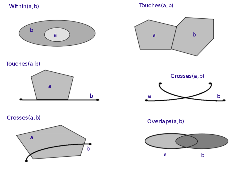
Lets explore these with Shapely!

We'll first set up some places and then see how their geometries interact.

In [127]:
# retrieve Belgium geometry from countries database

belgium = countries.loc[countries['NAME'] == 'Belgium', 'geometry'].unary_union
belgium
Out[127]:
In [128]:
# retrieve Paris geometry from cities database

paris = cities.loc[cities['NAME'] == 'Paris', 'geometry'].unary_union
paris
Out[128]:
In [129]:
# retrieve Brussels geometry from cities database

brussels = cities.loc[cities['NAME'] == 'Brussels', 'geometry'].unary_union
brussels
Out[129]:

Let's draw a line between Paris and Brussels:

In [130]:
# create line between cities

city_connect = shapely.geometry.LineString([paris, brussels])

Now we can plot everything:

In [131]:
# plot objects

gpd.GeoSeries([belgium, paris, brussels, city_connect]).plot(cmap='tab10');

We can easily test for geometric relations between objects, like in these examples below:

In [132]:
# check within

brussels.within(belgium)
Out[132]:
True
In [133]:
# check contains

belgium.contains(brussels)
Out[133]:
True
In [134]:
# check within

paris.within(belgium)
Out[134]:
False
In [135]:
# check contains

belgium.contains(paris)
Out[135]:
False

Similarly, a GeoDataFrame (and GeoSeries) will also take spatial relationships:

In [136]:
# find paris in countries database

countries[countries.contains(paris)]
Out[136]:
featurecla scalerank LABELRANK SOVEREIGNT SOV_A3 ADM0_DIF LEVEL TYPE ADMIN ADM0_A3 ... NAME_KO NAME_NL NAME_PL NAME_PT NAME_RU NAME_SV NAME_TR NAME_VI NAME_ZH geometry
22 Admin-0 country 0 2 France FR1 1 2 Country France FRA ... 프랑스 Frankrijk Francja França Франция Frankrike Fransa Pháp 法国 MULTIPOLYGON (((-54.11153 2.11427, -54.13491 2...

1 rows × 95 columns

In [137]:
# select Amazon river from rivers database

amazon = rivers[rivers['name'] == 'Amazonas'].geometry.unary_union
amazon
Out[137]:
In [138]:
# find countries that intersect Amazon river

countries[countries.intersects(amazon)]
Out[138]:
featurecla scalerank LABELRANK SOVEREIGNT SOV_A3 ADM0_DIF LEVEL TYPE ADMIN ADM0_A3 ... NAME_KO NAME_NL NAME_PL NAME_PT NAME_RU NAME_SV NAME_TR NAME_VI NAME_ZH geometry
4 Admin-0 country 0 2 Peru PER 0 2 Sovereign country Peru PER ... 페루 Peru Peru Peru Перу Peru Peru Peru 秘鲁 MULTIPOLYGON (((-69.51009 -17.50659, -69.63832...
45 Admin-0 country 0 2 Brazil BRA 0 2 Sovereign country Brazil BRA ... 브라질 Brazilië Brazylia Brasil Бразилия Brasilien Brezilya Brasil 巴西 MULTIPOLYGON (((-57.61170 -30.18296, -57.56865...
137 Admin-0 country 0 2 Colombia COL 0 2 Sovereign country Colombia COL ... 콜롬비아 Colombia Kolumbia Colômbia Колумбия Colombia Kolombiya Colombia 哥伦比亚 MULTIPOLYGON (((-78.82868 1.43431, -78.81286 1...

3 rows × 95 columns

In [139]:
# map countries that intersect Amazon

countries[countries.intersects(amazon)]['geometry']\
.append(gpd.GeoSeries(amazon)).plot(cmap='tab10');

Here is another example with the Danube:

In [140]:
# find and plot countries that intersect Danube river

danube = rivers[rivers['name'] == 'Danube'].geometry.unary_union
countries[countries.intersects(danube)]['geometry']\
.append(gpd.GeoSeries(danube),ignore_index=True).plot(cmap='tab10');

Performing Spatial Operations

Finally, we can perform spatial operations using Shapely. Let's look at a few examples:

In [141]:
# view amazon river

amazon
Out[141]:

Shapely makes it easy to create a buffer around a feature:

In [142]:
# create a buffer

super_amazon = amazon.buffer(10)
super_amazon
Out[142]:
In [143]:
# select Brazil from countries database

brazil = countries[countries['NAME']=='Brazil']['geometry'].unary_union
In [144]:
# plot Brazil, the Amazon river, and the buffer

gpd.GeoSeries([brazil, amazon, super_amazon]).plot(alpha=0.5, cmap='tab10');

Now we can view spatial relations between these polygons:

In [145]:
# intersects

super_amazon.intersection(brazil)
Out[145]:
In [146]:
# union

super_amazon.union(brazil)
Out[146]:
In [147]:
# union

brazil.union(super_amazon)
Out[147]:

Note that for some spatial relations, the order in which they are called matters.

In [148]:
# difference

super_amazon.difference(brazil)
Out[148]:
In [149]:
# difference

brazil.difference(super_amazon)
Out[149]:

Lets end with a few more examples.

In [150]:
# find countries in South America

countries[countries['CONTINENT'] == 'South America']
Out[150]:
featurecla scalerank LABELRANK SOVEREIGNT SOV_A3 ADM0_DIF LEVEL TYPE ADMIN ADM0_A3 ... NAME_KO NAME_NL NAME_PL NAME_PT NAME_RU NAME_SV NAME_TR NAME_VI NAME_ZH geometry
2 Admin-0 country 6 2 Chile CHL 0 2 Sovereign country Chile CHL ... 칠레 Chili Chile Chile Чили Chile Şili Chile 智利 MULTIPOLYGON (((-69.51009 -17.50659, -69.50611...
3 Admin-0 country 0 3 Bolivia BOL 0 2 Sovereign country Bolivia BOL ... 볼리비아 Bolivia Boliwia Bolívia Боливия Bolivia Bolivya Bolivia 玻利維亞 POLYGON ((-69.51009 -17.50659, -69.51009 -17.5...
4 Admin-0 country 0 2 Peru PER 0 2 Sovereign country Peru PER ... 페루 Peru Peru Peru Перу Peru Peru Peru 秘鲁 MULTIPOLYGON (((-69.51009 -17.50659, -69.63832...
5 Admin-0 country 0 2 Argentina ARG 0 2 Sovereign country Argentina ARG ... 아르헨티나 Argentinië Argentyna Argentina Аргентина Argentina Arjantin Argentina 阿根廷 MULTIPOLYGON (((-67.28475 -23.83414, -67.25133...
23 Admin-0 country 0 4 Suriname SUR 0 2 Sovereign country Suriname SUR ... 수리남 Suriname Surinam Suriname Суринам Surinam Surinam Suriname 蘇利南 POLYGON ((-54.08080 3.30931, -54.11429 3.28538...
24 Admin-0 country 0 4 Guyana GUY 0 2 Sovereign country Guyana GUY ... 가이아나 Guyana Gujana Guiana Гайана Guyana Guyana Guyana 圭亚那 MULTIPOLYGON (((-56.48182 1.94161, -56.52851 1...
45 Admin-0 country 0 2 Brazil BRA 0 2 Sovereign country Brazil BRA ... 브라질 Brazilië Brazylia Brasil Бразилия Brasilien Brezilya Brasil 巴西 MULTIPOLYGON (((-57.61170 -30.18296, -57.56865...
46 Admin-0 country 0 4 Uruguay URY 0 2 Sovereign country Uruguay URY ... 우루과이 Uruguay Urugwaj Uruguai Уругвай Uruguay Uruguay Uruguay 乌拉圭 POLYGON ((-53.37909 -33.74068, -53.39635 -33.7...
136 Admin-0 country 0 3 Ecuador ECU 0 2 Sovereign country Ecuador ECU ... 에콰도르 Ecuador Ekwador Equador Эквадор Ecuador Ekvador Ecuador 厄瓜多尔 MULTIPOLYGON (((-78.82868 1.43431, -78.76997 1...
137 Admin-0 country 0 2 Colombia COL 0 2 Sovereign country Colombia COL ... 콜롬비아 Colombia Kolumbia Colômbia Колумбия Colombia Kolombiya Colombia 哥伦比亚 MULTIPOLYGON (((-78.82868 1.43431, -78.81286 1...
138 Admin-0 country 0 4 Paraguay PRY 0 2 Sovereign country Paraguay PRY ... 파라과이 Paraguay Paragwaj Paraguai Парагвай Paraguay Paraguay Paraguay 巴拉圭 POLYGON ((-62.65036 -22.23446, -62.62752 -22.1...
158 Admin-0 country 0 3 Venezuela VEN 0 2 Sovereign country Venezuela VEN ... 베네수엘라 Venezuela Wenezuela Venezuela Венесуэла Venezuela Venezuela Venezuela 委內瑞拉 MULTIPOLYGON (((-60.02099 8.55801, -59.95969 8...
239 Admin-0 country 5 5 United Kingdom GB1 1 2 Dependency Falkland Islands FLK ... 포클랜드 제도 Falklandeilanden Falklandy Ilhas Malvinas Фолклендские острова Falklandsöarna Falkland Adaları Quần đảo Falkland 福克兰群岛 MULTIPOLYGON (((-59.69445 -52.20810, -59.67687...

13 rows × 95 columns

In [151]:
# find geometry for countries 

countries[countries['CONTINENT'] == 'South America'].unary_union
Out[151]:
In [152]:
# plot all countries

countries.plot(column='NAME', cmap='tab20c', figsize=(14,14), categorical=True);

Now go forth and explore!